
The following article involves utilizing association rule mining on a fictional store to find insights through identifying the interesting associations between the items sold in the store and provide suggestions to the owner.
Exploratory Data Analysis (EDA)
EDA in this context here refers to the processes of performing initial investigations on data so as to discover patterns, to spot anomalies, to test hypothesis and to check assumptions with the help of summary statistics and graphical representations. The insights from that are that Member 3308 is the store most frequent buyer, there are 3814 members registered with the store, 164 unique items sold and whole milk is the store’s most bought item. No apparent outliers are detected here. Further drilling down on the store’s top 50 most sold items can help to give us a sense of which items are more likely to end up in the association rules. This top 50 items shall give us a basis to work with when deciding the minimum support threshold which shall be explored later on. The top 50 sold items are illustrated below in Figure 1.
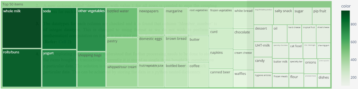 Figure 1: Treemap of Top 50 sold items
Preparation of Dataset
- Upon exploring the dataset, it is understood that further processing needs to be done to store the items bought as transactions. Currently it is stored as single items bought by members on a particular date. The solution is to group a list of items bought by each member on each particular date. This can be achieved by storing the data in a python nested dictionary and the code is shown below,
1
2
3
4
5
6
7
8
9
10
11
tem_dict = dict()                                  #dictionary to store the grouped data
                                                    #loop through each row of the dataframe
for i in df.values:                                 #store each row in a list format
    i = list(i)                                     #check if (i[0]=Member_number) is already present in the dictionary
    if i[0] in item_dict.keys():                    #check if (i[1]=Date) is already present under the Member_number
        if i[1] in item_dict[i[0]]:                 #if i[0] and i[1] are both present, append the items bought on that day
            item_dict[i[0]][i[1]].append(i[2])
        else:
            item_dict[i[0]].update({i[1]:[i[2]]})   #if i[1] is not present in in i[0], update the dictionary with the date and item bought
    else:
        item_dict[i[0]] = {i[1]:[i[2]]}
- Sample data stored in the dictionary can be seen below,
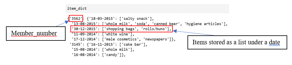 Figure 2: Sample data stored in the dictionary
- We shall not proceed to the next section unless ensuring no data are lost during the previous process. This can be done by simply looping through the dictionary and counting the cumulative length of the items list (inner most layer of the nested dictionary). They must be equal to the ‘count’ from .describe() function which is 19415. The code is shown below,
1
2
3
4
5
6
7
item_length = 0

for i in item_dict:
    for j in item_dict[i]:
        item_length = item_length + len(item_dict[i][j])

print('Total items in the dictionary are:', item_length)
- For the association rule mining algorithm library that will be used later on, the library requires all transactions to be stored as tuples in a list. We shall loop through the dictionary again for this step. An additional process will be incorporated where, data is first stored in a set before storing it in a tuple. This is to ensure no duplicates are present within the same transaction. A length check will also be done to quantify the number of duplicates. The code is shown below,
1
2
3
4
5
6
7
8
9
10
11
transactions = list()
transactions_length = 0

for i in item_dict:
    for j in item_dict[i]:
        transactions.append(tuple(set(item_dict[i][j])))

for i in transactions:
    transactions_length = transactions_length + len(i)

print('Total items in the tuple accounting for duplicates are:', transactions_length)
- From the previous step, it is understood that 19415 – 19250 = 165 items were present as duplicates in the dataset. The dataset is now in a format that is usable for association rule mining.
Methodology
The method that will be used for mining the association rule here is the A-Priori Algorithm. According to (Kantardzic, 2020), A-Priori Algorithm can be understood as the computation of frequent itemsets in a database through multiple iterations by the process of ‘candidate generation’ and ‘candidate counting and selection’ in each iteration and ending with itemsets above a certain threshold considered frequent. To ensure interesting rules, the minimum threshold shall be selected based on mathematical justification.
From the initial EDA, most sold item is ‘whole milk’ with 947 counts. Calculating it’s support would give us, 947/19415 ≈4.9%. This means that any number higher than 4.9% = 0.049 will not generate any rules. For the purposes of this project and to ensure a comprehensive analysis, we first get the support for the top 50 items sold. This is to ensure the incorporation of more interesting rules as just limiting the analysis to the top 10 items sold has no guarantee of generating association rules.
The support for 50th item sold is approximately 104/19250 = 0.005. The method that shall be employed here is by splitting 0.005 into 10 intervals. Excluding 0, each interval will be added by 0.005 and iterated through the apriori algorithm and the length of the rules generated will be stored in a dictionary. A manual judgement shall then take place on which minimum support threshold to use. The code block for these steps can be viewed below,
1
2
3
4
5
6
7
8
maximum = (df_table['item_count'].loc[50])/transactions_length
minimum = 0
interval = (maximum - minimum)/10
minimum_support = list()

for i in range(9):
    minimum = minimum + interval
    minimum_support.append(round(minimum, 4))
1
2
3
4
5
6
7
8
9
from efficient_apriori import apriori

support_dict = dict()

min_confidence = 0      # For now set min_confidence = 0 to obtain all the rules

for support in minimum_support:
    itemsets, rules = apriori(transactions, min_support=support, min_confidence=min_confidence)
    support_dict[support] = len(rules)
From the previous step, the maximum support specified in the list which is 0.0049 generated 0 rules. To ensure inclusiveness, we shall go with the minimum support threshold of 0.0005 to generate 478 rules in total and further filtering will take place based on rule metrics later on. As for the minimum confidence level, we shall again stick with 0 as we have no intuition on the distribution of confidence among the rules generated.
For efficient_apriori library, the resulting rules are generated as strings stored in a list. This would be very hard to get any valuable insights on. As a result for this, further data processing shall take place to store the data in a dataframe or a tabular format. The first 5 rows of the resulting dataframe are illustrated below in Figure 3.
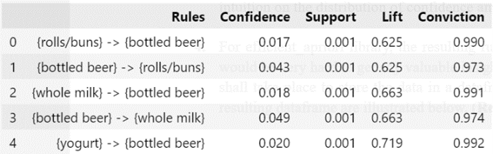
In terms of rules interpretation or performance measure, there are 4 main metrics that shall be evaluated. They are support, confidence, lift and conviction. Support can be understood as simply the proportion of the itemset in all transactions or how much frequent it is. Confidence is the measure that informs us how likely a consequent item is purchased when an antecedent item is purchased, or simply put as {X -> Y}. The value ranges from 0 to 1 which can be translated in percentages. The con for confidence measure is that it only takes into account of how popular item X is.
- An additional measure to account for association between the itemsets is lift. Using the {X -> Y} convention from the previous step, lift can be understood as the likelihood of Y being purchased when item X is purchased while controlling for how popular item Y is. The values of lift can be interpreted as below:
Lift < 1: Y is unlikely to be bought if X is bought
Lift = 1: Y and X has no association
Lift > 1: Y is likely to be bought if X is bought - The final performance measure that shall be employed is conviction. According to (Azevedo & Jorge, 2007), conviction is a measure to combat the weakness of both confidence and lift while being sensitive to rule direction which means that (conv(X -> Y) ≠ conv(Y -> X)). Interpretation of the values of conviction are as below:
Conviction = ∞: Logical implications (confidence=1)
Conviction = 1: Y and X has no association
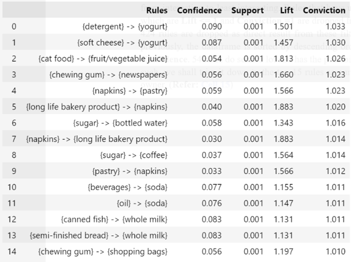
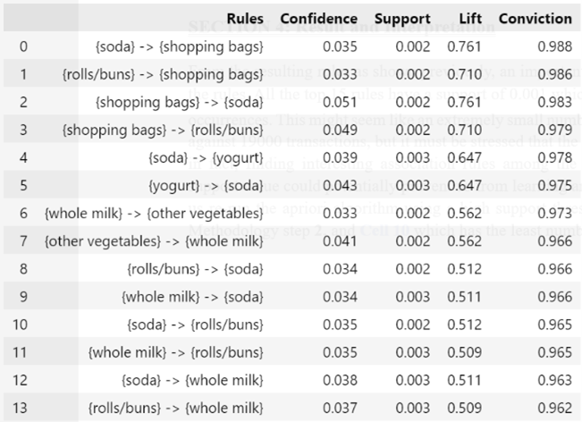
Conviction > 1: Y is likely to be bought if X is bought - Using the previous 3 steps as a basis, we shall form a hierarchy of ranking to filter and sort the rules from interesting to least interesting. Rules that have unlikely or no association between them which are Lift <= 1 and Conviction =1 are dropped from the dataframe. A total of 478 – 54 = 424 rules are dropped as direct result from these filters. Alluding to the mentioned ranking previously, the dataframe is sorted by descending order and obeying the rank of Conviction > Lift > Confidence. 54 rules do seem a lot and has the possibility of containing uninteresting rules. As such, we shall trim it down to the top 15 rules as our basis for recommendations to the store owner and is shown in Figure 4 below,
Result and Interpretation
From the resulting rules as shown previously, an important metric must be addressed to make sense of the rules. All the top 15 rules have a support of 0.001 which translates roughly to 0.001 x 19250 ≈ 19 occurrences. This might seem like an extremely small number of occurrences especially when compared against 19000 transactions, but it must be stressed that the goal here is not to find frequent itemsets but in fact, finding interesting association rules among the transactions. Similarly, all the confidence values are below 10%. This can be explained by the formula of confidence itself, support({Y})/support ({X}). Mathematically speaking for this case, where high confidence values are values ≈ 1, it is possible only if the positive difference between numerator and denominator is as small as possible. Since the minimum support threshold (numerator) is set to a very low level, the confidence levels are bound to be low as the denominator (antecedent support) will be bigger compared to the numerator. Prioritizing a high minimum support value could potentially prevent us from learning any interesting associations. To prove this, let us re-run the apriori algorithm using a high support threshold, in this case it would be 0.0022 from Methodology step 2. which has the least number of rules. The result is shown in Figure 5 below,
As we can see above, even though the support is higher, none of the rules has lift and conviction more than 1, rendering them as an unlikely association and will be unwise to recommend them to the store owner. Going back to the top 15 association rules from Methodology step 9., some of the recommendations that the store owner could exploit in placement of the items are,
- Placing detergent, soft cheese and yogurt in close proximity to one another.
- Placing fruit/vegetable juice near to cat food.
- Placing chewing gum, newspapers and shopping bags close to each other.
- Placing long life bakery product, napkins, pastry in the same location.
- Placing sugar, bottled water and coffee near to each other.
- Placing beverages, oil and soda in the same location.
- Placing semi-finished bread, canned fish and whole milk in close proximity to one another.
It must be noted that although the generated rules are of length 2 (2 items in one rule), the recommendations are mentioning 3 items together. This is because some rules are related by a common item and by taking advantage of it, item sales might improve. Should the store owner implement the recommendations, it would be advised for the store owner to provide future sales data as well to verify the validity of the association rules and to suggest further tweaks based on the data if necessary.
References
Azevedo, P., & Jorge, A. (2007). Comparing Rule Measures for Predictive Association Rules. 4701. 510-517. Machine Learning: ECML 2007. https://link.springer.com/chapter/10.1007/978-3-540-74958-5_47
Kantardzic, M. (2020). Data Mining: Concepts, Models, Methods, and Algorithms (3rd. ed.). Wiley-IEEE Press. https://dl.acm.org/doi/10.5555/2073641
The raw dataset, Python notebook to run A-priori algorithm, and the generated association rules mentioned in this article are hosted in my Github Repo.