The following article shows the step-by-step process on performing sentiment analysis on movie reviews. The datasets used in this project are from Kaggle should you want to follow along.
- Step 1: Import primary dataset
1
2
3
| import pandas as pd
df_movies = pd.read_csv('rotten_tomatoes_movies.csv')
|
- Step 2: Check columns and data types
- Step 3: Remove unecessary columns
1
2
| df_movies = df_movies[['rotten_tomatoes_link', 'movie_title',
'directors', 'production_company']]
|
- Step 4: Check counts of null values
1
2
| null_counts = df_movies.isnull().sum() #check counts of null values
null_counts
|
- Step 5: Replace null values with N/A
1
2
3
| df_movies.fillna('N/A', inplace=True)
null_counts = df_movies.isnull().sum()
null_counts
|
- Step 6: Drop any available duplicates in rotten tomatoes link
1
2
| df_movies.drop_duplicates(subset=['rotten_tomatoes_link'],
keep='last', inplace=True)
|
- Step 7: Import Secondary Dataset (which includes the movie reviews)
1
| df_movies_review = pd.read_csv('rotten_tomatoes_critic_reviews.csv')
|
- Step 8: Removal of unnecessary columns and Initial EDA
1
2
3
| df_movies_review = df_movies_review[['rotten_tomatoes_link', 'critic_name',
'review_type', 'review_content']]
df_movies_review.describe(include='all')
|
- Step 9: Remove rows with empty reviews, replace all other empty rows with N/A
1
2
3
4
| df_movies_review = df_movies_review[df_movies_review['review_content'].notna()]
df_movies_review.fillna('N/A', inplace=True)
null_counts=df_movies_review.isnull().sum()
null_counts
|
- Step 10: Merge primary and secondary dataset by a common key, rotten_tomatoes_link
1
| df = pd.merge(df_movies_review, df_movies, how='inner', on='rotten_tomatoes_link')
|
- Step 11: Check for null values and drop any duplicates on review content
1
2
3
| df.drop_duplicates(subset=['review_content'], keep='last', inplace=True)
null_counts = df.isnull().sum() #check counts of null values
null_counts
|
- Step 12: On review type, change Fresh to Positive, Rotten to Negative
1
2
| df['review_type'] = df['review_type'].replace(['Fresh'], 'Positive')
df['review_type'] = df['review_type'].replace(['Rotten'], 'Negative')
|
- Step 13: Cleaning the texts
1
2
3
4
5
6
7
8
9
10
11
| import re
# Define a function to clean the text
def clean(text):
# Removes all special characters and numericals leaving the alphabets
text = re.sub('[^A-Za-z]+', ' ', text)
return text
# Cleaning the text in the review column
df['cleaned_reviews'] = df['review_content'].apply(clean)
df.head()
|
Figure 1: Snippet of cleaned reviews
- Step 14: Tokenization, POS Tagging, Stopwords Removal
1
2
3
4
5
6
7
8
9
10
11
12
13
14
15
16
17
18
19
20
21
22
23
24
25
26
27
28
| import nltk
nltk.download('punkt')
nltk.download('omw-1.4')
nltk.download('averaged_perceptron_tagger')
from nltk.tokenize import word_tokenize
from nltk import pos_tag
nltk.download('stopwords')
from nltk.corpus import stopwords
nltk.download('wordnet')
from nltk.corpus import wordnet
from tqdm import tqdm
# POS tagger dictionary
pos_dict = {'J':wordnet.ADJ, 'V':wordnet.VERB, 'N':wordnet.NOUN, 'R':wordnet.ADV}
# Define a function to tokenize, POS tag and remove stopwords in the form of a tuple
def token_stop_pos(text):
tags = pos_tag(word_tokenize(text))
newlist = []
for word, tag in tags:
if word.lower() not in set(stopwords.words('english')):
newlist.append(tuple([word, pos_dict.get(tag[0])]))
return newlist
# Apply the token function in the reviews column
tqdm.pandas(desc='POS_tagged')
df['POS_tagged'] = df['cleaned_reviews'].progress_apply(token_stop_pos)
df.head()
|
Figure 2: Snippet of POS tagged reviews
- Step 15: Obtaining stem words
1
2
3
4
5
6
7
8
9
10
11
12
13
14
15
16
17
18
19
| from nltk.stem import WordNetLemmatizer
wordnet_lemmatizer = WordNetLemmatizer()
# Define a function for lemmatization process
def lemmatize(pos_data):
lemma_rew = " "
for word, pos in pos_data:
if not pos:
lemma = word
lemma_rew = lemma_rew + " " + lemma
else:
lemma = wordnet_lemmatizer.lemmatize(word, pos=pos)
lemma_rew = lemma_rew + " " + lemma
return lemma_rew
# Apply the lemmatize function in the POS_tagged column
tqdm.pandas(desc='Lemma')
df['Lemma'] = df['POS_tagged'].progress_apply(lemmatize)
df.head()
|
Figure 3: Snippet of Lemmatized reviews
- Step 15: Sentiment analysis using TextBlob
1
2
3
4
5
6
7
8
9
10
11
12
13
14
15
16
17
18
19
20
21
22
23
24
25
26
27
28
29
| from textblob import TextBlob
# function to calculate subjectivity
def getSubjectivity(review):
return TextBlob(review).sentiment.subjectivity
# function to calculate polarity
def getPolarity(review):
return TextBlob(review).sentiment.polarity
# function to analyze the reviews
def analysis(score):
if score < 0:
return 'Negative'
elif score == 0:
return 'Neutral'
else:
return 'Positive'
tqdm.pandas(desc='Subjectivity')
df['Subjectivity'] = df['Lemma'].progress_apply(getSubjectivity)
tqdm.pandas(desc='Polarity')
df['Polarity'] = df['Lemma'].progress_apply(getPolarity)
tqdm.pandas(desc='Textblob Analysis')
df['textblob_analysis'] = df['Polarity'].progress_apply(analysis)
df.head()
|
Figure 4: Snippet of Sentiment Analysis on reviews
- Step 16: Accuracy of the sentiment analysis. It was 0.578 in this case
1
2
3
| from sklearn.metrics import accuracy_score
accuracy_score(df['review_type'], df['textblob_analysis'])
|
- Step 17: Further Data Processing (Compare review labels vs textblob_analysis, Drop all false values)
1
2
3
4
5
6
7
8
9
10
11
12
13
14
| import numpy as np
conditions = [
(df['review_type'] == df['textblob_analysis']),
((df['review_type'] == 'Negative') & (df['textblob_analysis'] == 'Positive')),
((df['review_type'] == 'Positive') & (df['textblob_analysis'] == 'Neutral')),
((df['review_type'] == 'Negative') & (df['textblob_analysis'] == 'Neutral'))
]
values = ['True', 'False', 'True', 'False']
df['review_check'] = np.select(conditions, values)
df.drop(df[df['review_check'] == 'False'].index, inplace=True)
df.drop(['review_check'], axis=1, inplace=True)
df = df.reset_index(drop=True)
|
- Step 18: Visualize Proportion of Sentiments
1
2
3
4
5
6
7
8
9
10
11
12
| import matplotlib.pyplot as plt
import seaborn as sns
df['count'] = 1
df_table = pd.DataFrame(df.groupby('textblob_analysis')['count'].sum().sort_values(ascending=False).reset_index())
colours = sns.color_palette('pastel')
labels = ['Positive', 'Neutral', 'Negative']
plt.pie(df_table['count'], labels=labels, colors=colours, autopct='%.2f%%')
plt.title("Proportion of Sentiments")
plt.show()
|
Figure 5: Proportion of Sentiments
- Step 19: Visualize Sentiment Distribution of Movies
1
2
3
4
5
6
7
8
9
10
11
12
13
14
15
16
17
18
| df_movie = df.groupby(['movie_title', 'textblob_analysis'],
as_index=False)['count'].sum().sort_values(by=['count'],
ascending=False).reset_index(drop=True)
df_movie_positive = df_movie.query('textblob_analysis == "Positive"').head(10).reset_index(drop=True)
df_movie_neutral = df_movie.query('textblob_analysis == "Neutral"').head(10).reset_index(drop=True)
df_movie_negative = df_movie.query('textblob_analysis == "Negative"').head(10).reset_index(drop=True)
fig, axes = plt.subplots(1, 3, figsize=(20, 6))
fig.suptitle('Top Sentiment Distribution of Movies')
sns.barplot(ax=axes[0], x='count', y='movie_title', data=df_movie_positive,
palette = ("BuGn_r"), orient='h').set(title='Positive Sentiment')
sns.barplot(ax=axes[1], x='count', y='movie_title', data=df_movie_negative,
palette = 'OrRd_r', orient='h').set(title='Negative Sentiment')
sns.barplot(ax=axes[2], x='count', y='movie_title', data=df_movie_neutral,
palette = 'Blues_r', orient='h').set(title='Neutral Sentiment')
plt.tight_layout()
plt.show()
|
Figure 6: Top Sentiment Distribution of Movies
- Step 19: Visualize Sentiment Distribution of Directors
1
2
3
4
5
6
7
8
9
10
11
12
13
14
15
16
17
18
19
| df_directors = df.groupby(['directors', 'textblob_analysis'],
as_index=False)['count'].sum().sort_values(by=['count'],
ascending=False).reset_index(drop=True)
df_directors.drop(df_directors[df_directors['directors'] == 'N/A'].index, inplace=True)
df_directors_positive = df_directors.query('textblob_analysis == "Positive"').head(10).reset_index(drop=True)
df_directors_neutral = df_directors.query('textblob_analysis == "Neutral"').head(10).reset_index(drop=True)
df_directors_negative = df_directors.query('textblob_analysis == "Negative"').head(10).reset_index(drop=True)
fig, axes = plt.subplots(1, 3, figsize=(20, 6))
fig.suptitle('Top Sentiment Distribution of Directors')
sns.barplot(ax=axes[0], x='count', y='directors', data=df_directors_positive,
palette = ("BuGn_r"), orient='h').set(title='Positive Sentiment')
sns.barplot(ax=axes[1], x='count', y='directors', data=df_directors_negative,
palette = 'OrRd_r', orient='h').set(title='Negative Sentiment')
sns.barplot(ax=axes[2], x='count', y='directors', data=df_directors_neutral,
palette = 'Blues_r', orient='h').set(title='Neutral Sentiment')
plt.tight_layout()
plt.show()
|
Figure 7: Top Sentiment Distribution of Directors
- Step 19: Visualize Sentiment Distribution of Production Companies
1
2
3
4
5
6
7
8
9
10
11
12
13
14
15
16
17
18
19
| df_production = df.groupby(['production_company', 'textblob_analysis'],
as_index=False)['count'].sum().sort_values(by=['count'],
ascending=False).reset_index(drop=True)
df_production.drop(df_production[df_production['production_company'] == 'N/A'].index, inplace=True)
df_production_positive = df_production.query('textblob_analysis == "Positive"').head(10).reset_index(drop=True)
df_production_neutral = df_production.query('textblob_analysis == "Neutral"').head(10).reset_index(drop=True)
df_production_negative = df_production.query('textblob_analysis == "Negative"').head(10).reset_index(drop=True)
fig, axes = plt.subplots(1, 3, figsize=(20, 6))
fig.suptitle('Top Sentiment Distribution of Production Companies')
sns.barplot(ax=axes[0], x='count', y='production_company', data=df_production_positive,
palette = ("BuGn_r"), orient='h').set(title='Positive Sentiment')
sns.barplot(ax=axes[1], x='count', y='production_company', data=df_production_negative,
palette = 'OrRd_r', orient='h').set(title='Negative Sentiment')
sns.barplot(ax=axes[2], x='count', y='production_company', data=df_production_neutral,
palette = 'Blues_r', orient='h').set(title='Neutral Sentiment')
plt.tight_layout()
plt.show()
|
Figure 8: Top Sentiment Distribution of Production Companies
- Step 20: Visualize Sentiment Distribution of Critics
1
2
3
4
5
6
7
8
9
10
11
12
13
14
15
16
17
18
19
| df_critic = df.groupby(['critic_name', 'textblob_analysis'],
as_index=False)['count'].sum().sort_values(by=['count'],
ascending=False).reset_index(drop=True)
df_critic.drop(df_critic[df_critic['critic_name'] == 'N/A'].index, inplace=True)
df_critic_positive = df_critic.query('textblob_analysis == "Positive"').head(10).reset_index(drop=True)
df_critic_neutral = df_critic.query('textblob_analysis == "Neutral"').head(10).reset_index(drop=True)
df_critic_negative = df_critic.query('textblob_analysis == "Negative"').head(10).reset_index(drop=True)
fig, axes = plt.subplots(1, 3, figsize=(20, 6))
fig.suptitle('Top Sentiment Distribution of Critics')
sns.barplot(ax=axes[0], x='count', y='critic_name', data=df_critic_positive,
palette = 'BuGn_r', orient='h').set(title='Positive Sentiment')
sns.barplot(ax=axes[1], x='count', y='critic_name', data=df_critic_negative,
palette = 'OrRd_r', orient='h').set(title='Negative Sentiment')
sns.barplot(ax=axes[2], x='count', y='critic_name', data=df_critic_neutral,
alette = 'Blues_r', orient='h').set(title='Neutral Sentiment')
plt.tight_layout()
plt.show()
|
Figure 9: Top Sentiment Distribution of Critics
- Step 21: Visualize Top Words used in the Sentiments
1
2
3
4
5
6
7
8
9
10
11
12
13
14
15
16
17
18
19
20
21
22
23
24
25
26
27
28
29
30
31
32
33
34
35
36
37
38
39
| from wordcloud import WordCloud, STOPWORDS
df_positive = df.query("textblob_analysis == 'Positive'").reset_index(drop=True)
positive_text = ' '.join(word.lower() for word in df_positive['cleaned_reviews'])
df_negative = df.query("textblob_analysis == 'Negative'").reset_index(drop=True)
negative_text = ' '.join(word.lower() for word in df_negative['cleaned_reviews'])
df_neutral = df.query("textblob_analysis == 'Neutral'").reset_index(drop=True)
neutral_text = ' '.join(word.lower() for word in df_neutral['cleaned_reviews'])
stopwords = set(STOPWORDS)
stopwords.update(['movie', 'film', 'story', 'character', 's', 'one', 'make',
'even', 't', 'work', 'time', 'feel', 'characters'])
fig, axes = plt.subplots(1, 3, figsize=(20, 6))
fig.suptitle('Top Words used in the Sentiments')
wordcloud1 = WordCloud(stopwords=stopwords, background_color="white",
colormap='Greens').generate(positive_text)
wordcloud2 = WordCloud(stopwords=stopwords, background_color="white",
colormap='Oranges').generate(negative_text)
wordcloud3 = WordCloud(stopwords=stopwords, background_color="white",
colormap='Blues').generate(neutral_text)
axes[0].imshow(wordcloud1, interpolation='bilinear')
axes[0].set_title('Top Positive Words')
axes[0].set_axis_off()
axes[1].imshow(wordcloud2, interpolation='bilinear')
axes[1].set_title('Top Negative Words')
axes[1].set_axis_off()
axes[2].imshow(wordcloud3, interpolation='bilinear')
axes[2].set_title('Top Neutral Words')
axes[2].set_axis_off()
plt.tight_layout()
plt.show()
|
Figure 10: Top Words used in the sentiments
The Python notebook for the sentiment analysis mentioned in this article is hosted in my Github Repo.

 Figure 1: Snippet of cleaned reviews
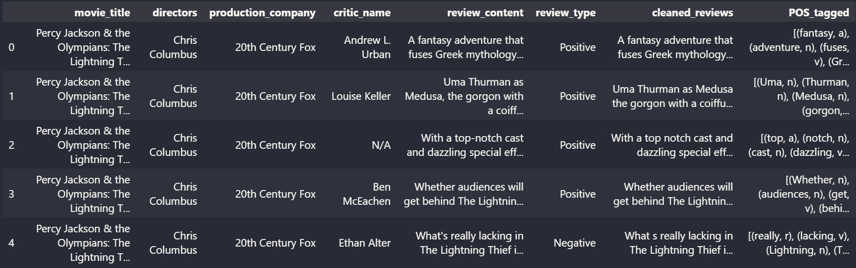 Figure 2: Snippet of POS tagged reviews
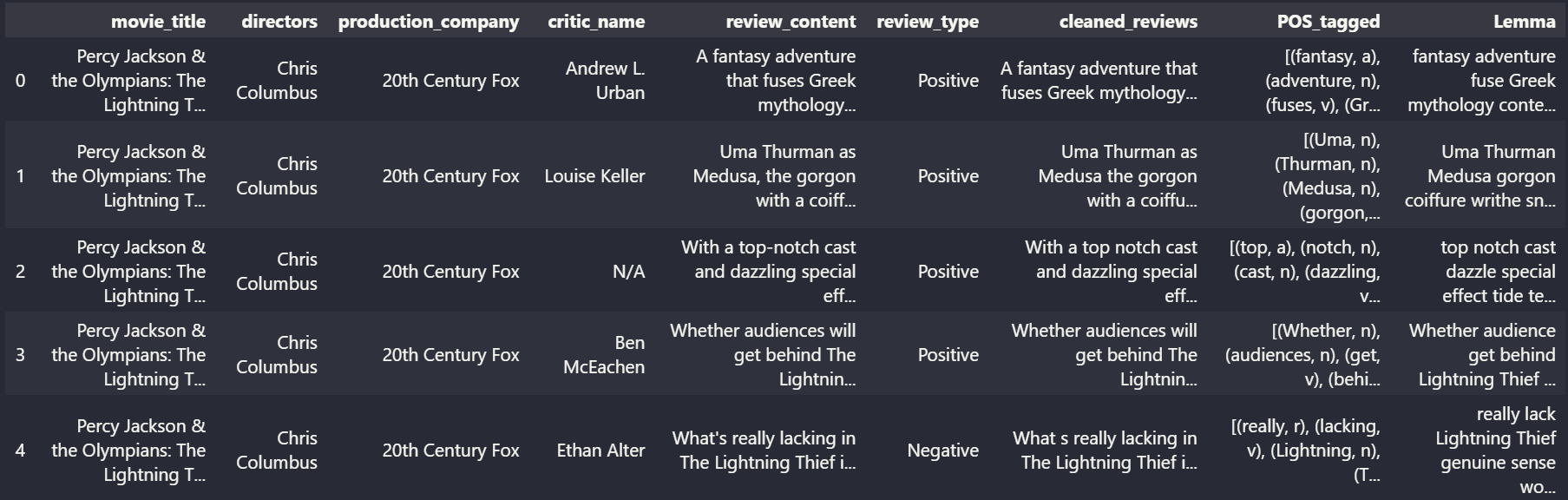 Figure 3: Snippet of Lemmatized reviews
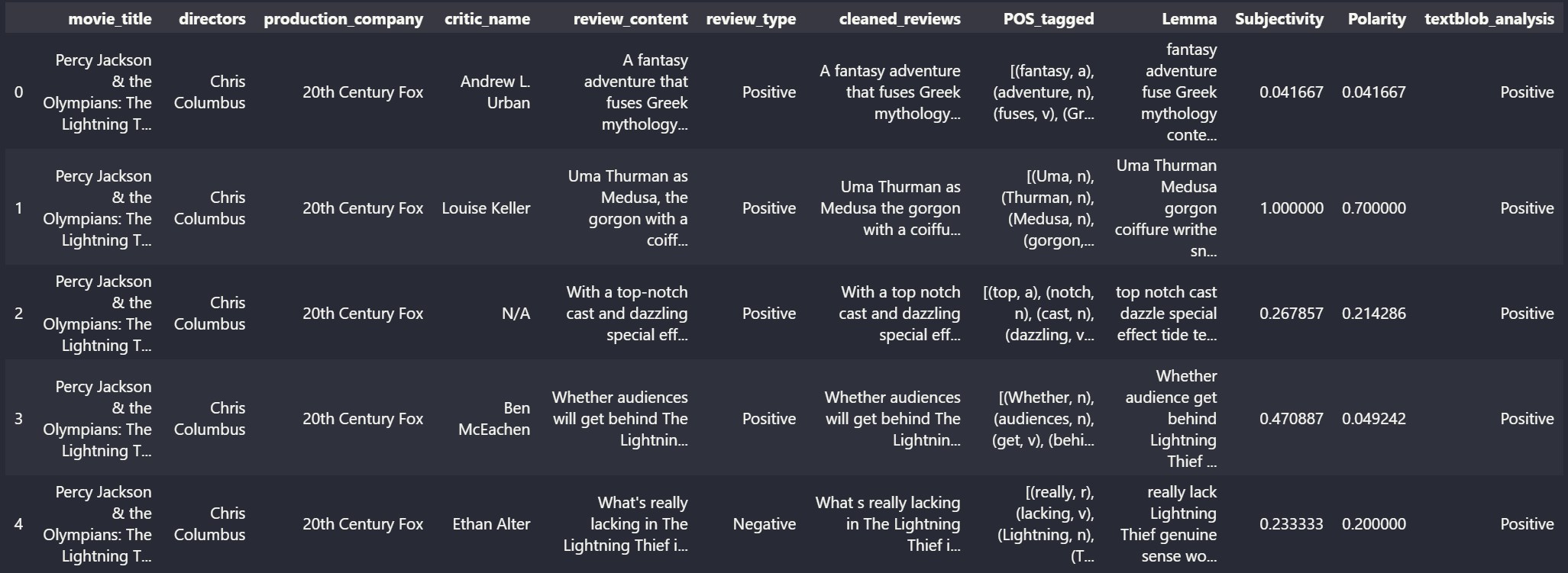 Figure 4: Snippet of Sentiment Analysis on reviews
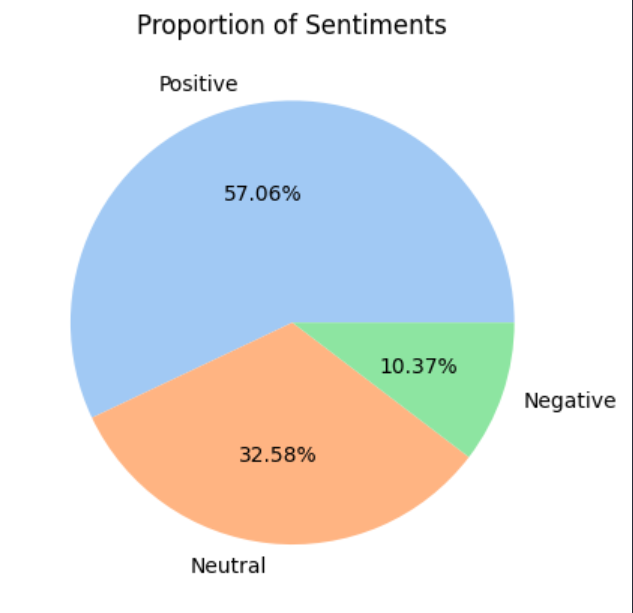 Figure 5: Proportion of Sentiments
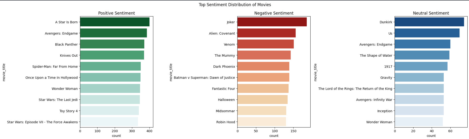 Figure 6: Top Sentiment Distribution of Movies
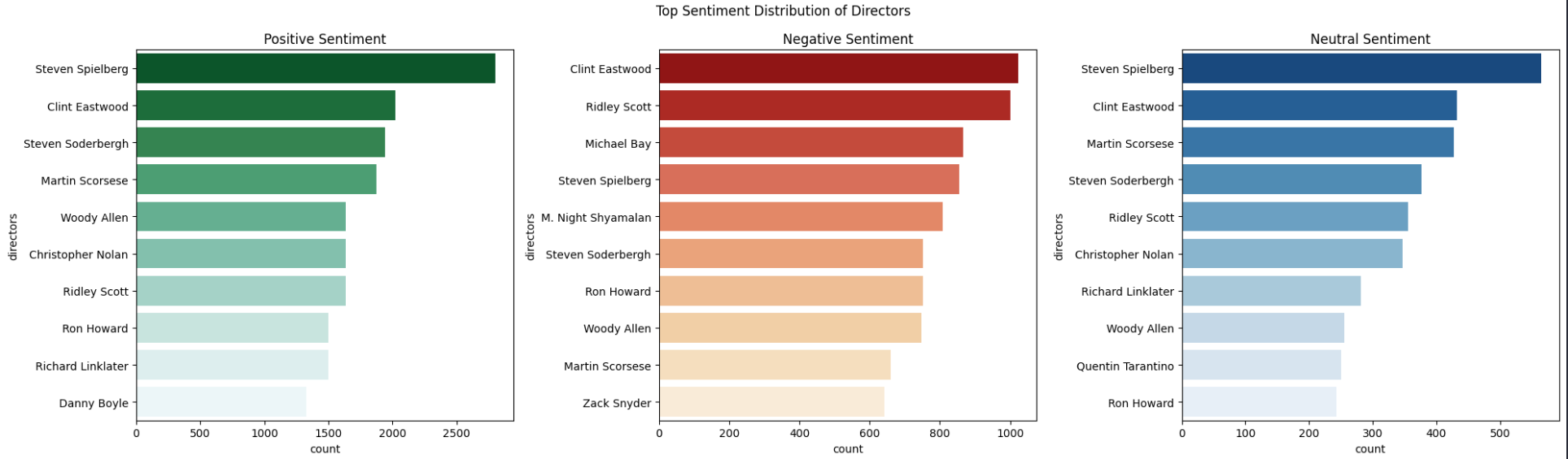 Figure 7: Top Sentiment Distribution of Directors
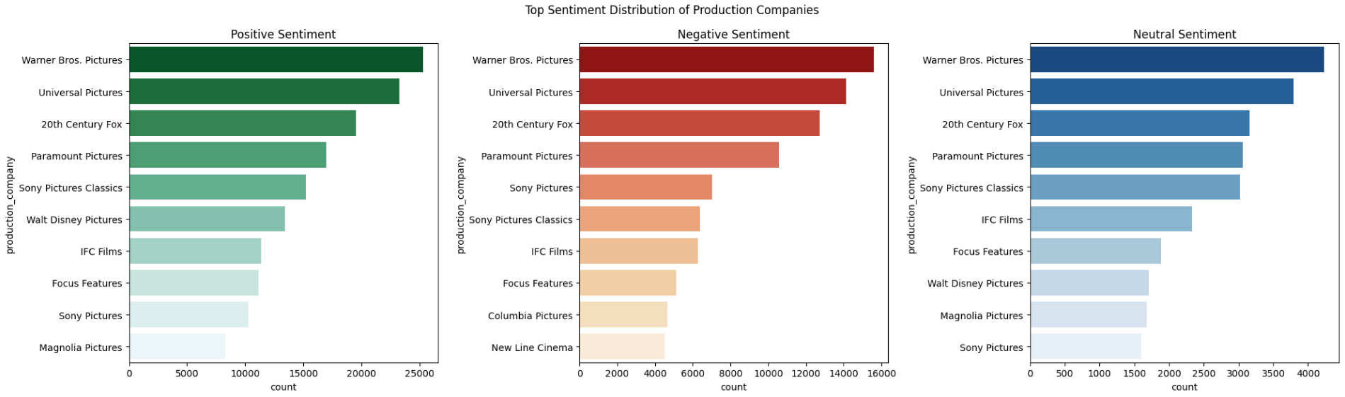 Figure 8: Top Sentiment Distribution of Production Companies
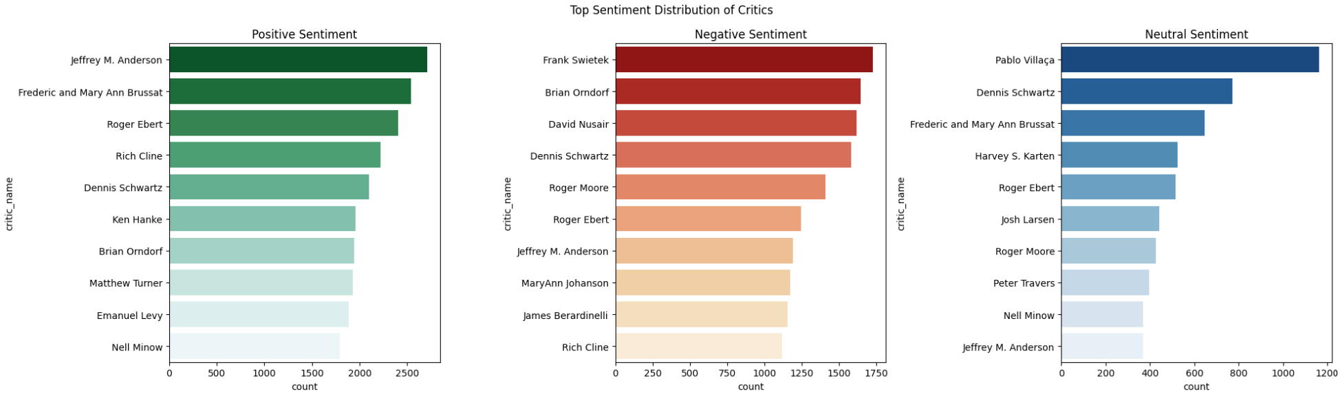 Figure 9: Top Sentiment Distribution of Critics
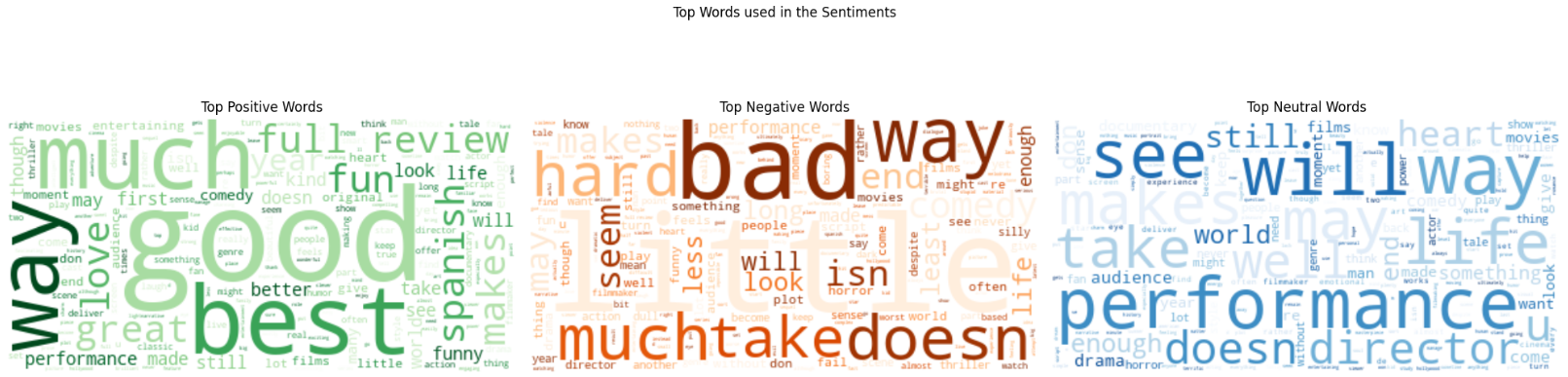 Figure 10: Top Words used in the sentiments