Crime Rate Machine Learning Prediction Model in England

The following article discusses the steps taken in developing fairly accurate ML models in predicting crime rates in England. It shall also cover the outcomes of the initial ML models in terms of their performance, testing, validation, as well as the analysis and evaluation of the final ML models.The datasets involved in this project can be accessed via the posts below,

• Crime Incidents
• Deprivation Index Data
• Unemployment Rate
• Population Density
• Crime Rate

Data Merging

Before proceeding with the ML development, the datasets needs to be merged into a single tabular file where all the predicting features and target feature (Crime Rate) resides. The steps to achieve this objective can be viewed in the code block below and the snippet of the merged dataset is shown in Figure 1.

import pandas as pd

#Load all required datasets into a Pandas DataFrame
df_crimerate = pd.read_csv('2011-2022_crimerate.csv')
df_deprivation = pd.read_csv('2011-2022_deprivation.csv')
df_inflation = pd.read_csv('2011-2022_inflationrate.csv')
df_unemployment = pd.read_csv('2011-2022_unemployment.csv')

#Merge all DataFrames into a single DataFrame
df_crimerate = pd.merge(df_crimerate, df_deprivation, on=['Month', 'LSOA code'], how='left')
df_crimerate = pd.merge(df_crimerate, df_inflation, on='Month', how='left')
df_crimerate = pd.merge(df_crimerate, df_unemployment, on='Month', how='left')
df_crimerate = df_crimerate.drop(['Month', 'LSOA code', 'Count', 'AS Score', 'Inflation_rate', 'Indoors Score'], axis=1)

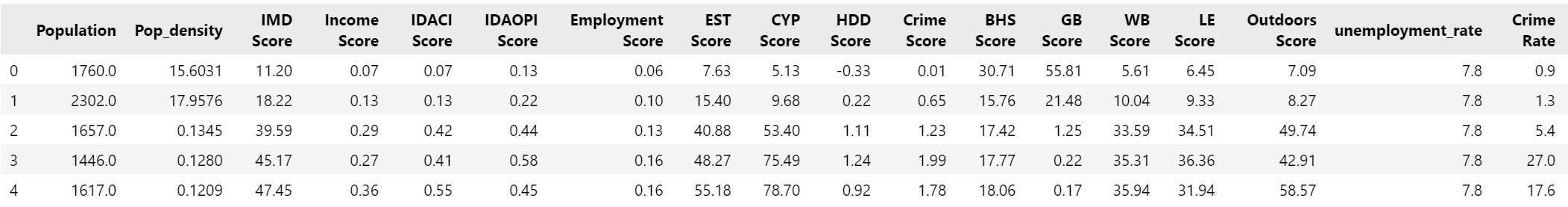Figure 1: Snippet of Merged Crime Rate

Initial ML Models Development

There are 5 initial ML models chosen for this project in the hopes of producing the best results. The initial ML models and its corresponding parameters are as below. All parameters are left to default settings unless otherwise stated.

1. Random Forest Regression: n_jobs=-1, max_depth=8
2. Decision Tree Regression: max_depth=8
3. Extra-Trees Regression: max_depth=8
4. Linear Regression: n_jobs=-1
5. XGBoost Regression: tree_method=’gpu_hist’, max_depth=8

Setting n_jobs to -1 essentially means to use all available CPU threads. tree_method=’gpu_hist’ in XGBoost takes advantage of CUDA computing in GPU to achieve blazingly fast performance as shall be explored later on.

Initial ML Models Performance

A benchmarking script was developed in Python to measure the initial performance of all five models. The performance results are presented visually in Figure 2 below.

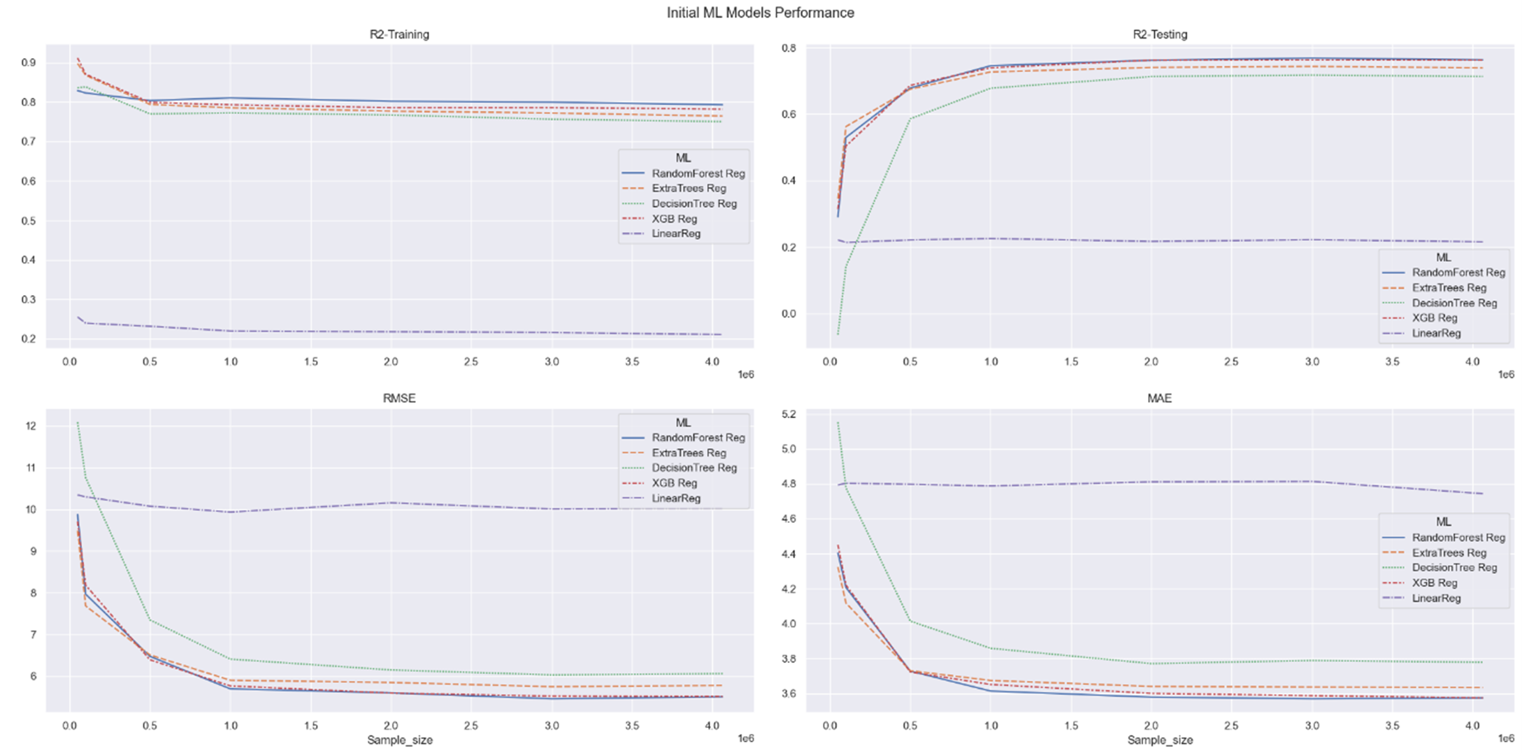Figure 2: Initial ML Models Performance

Based on the charts shown in Figure 2, it is evident that the Random Forest Regressor and XGBoost Regressor excel in performance across all four metrics. In particular, these two models consistently achieve the highest R² scores for both training and testing, indicating their superior performance across different sample sizes. Furthermore, when considering the evaluation of RMSE and MAE, which measure the errors between predicted and actual values, Random Forest and XGBoost consistently demonstrate the lowest values across all sample sizes, further highlighting their superiority. While the Decision Tree Regression and Extra Tree Regression models exhibit similar trends to Random Forest and XGBoost, their performance falls significantly behind in terms of R² scores and error metrics. Lastly, Linear Regression proves to be the least effective model across all four evaluated metrics. The comparison of performance over time for the ML models is depicted in Figure 3 below.

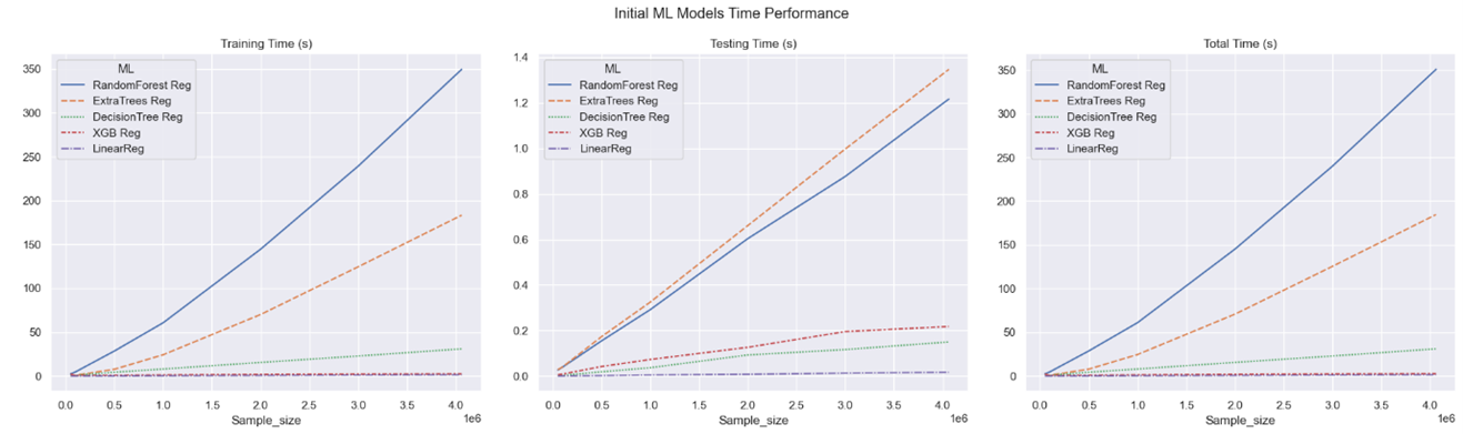Figure 3: Initial ML Models Time Performance

In addition to performance evaluation metrics, considering the training, testing, and total time of machine learning models provides an important aspect in assessing overall model quality. Figure 3 presents the varying time consumption of different models, highlighting XGBoost’s impressive performance with the lowest total time while also excelling in other evaluation metrics. On the other hand, despite Random Forest’s strong performance in evaluation metrics, it is the least efficient among the five models, taking approximately 175% longer than XGBoost when using the complete dataset. This difference can be attributed to the computational nature of the algorithms, where XGBoost utilizes GPU, while Random Forest relies on CPU. After carefully analyzing the data shown in Figure 2 and Figure 3, the XGBoost Regression model has been chosen for the upcoming testing and validation stage due to its impressive performance, as it yields minimal errors while minimizing computational time. Furthermore, despite its longer computation duration, the Random Forest Regression model has also been selected for its superior performance in evaluation metrics.

Random Forest Regression GridSearchCV

As shown in Figure 3, the training time for the Random Forest Regression model grows proportionally with the sample size. Specifically, it takes around 350 seconds to train the model using the entire dataset. To provide context, it’s worth mentioning that training a GridSearchCV model with 4 hyperparameters, each having 3 possible values, and applying 5-fold cross-validation to the complete dataset would result in a training time of 3 x 3 x 3 x 3 x 5 x 350s = 141750s. When converted to hours, the mentioned duration corresponds to approximately 39 hours, which is a significant amount of time required for training a GridSearchCV model. Therefore, additional optimization techniques are necessary to reduce computation time while maintaining similar levels of quality. As shown in Figure 2, the R² scores and error values start to stabilize after a certain sample size. This suggests that training a subset of the dataset, rather than the entire dataset, could yield comparable results while minimizing the training duration. Specifically, Figure 2 indicates that this stabilization occurs at 1 million samples. Consequently, choosing to train the GridSearchCV model with this sample size would result in,

1. The reduction in size from the original dataset to the sampling data is 100% - ((1000000/4062364) x 100%) = 75.38%.
2. Estimated training time using the previous example is 3 x 3 x 3 x 3 x 5 x 60 = 24300 seconds = 6.75 hours. The improvement in training time can be quantified to approximately, ((6.75 – 39) / 39) x 100% = 82.7%.

In developing the GridSearchCV (Random Forest Regression) model, the hyperparameters that are selected are as below,

1. n_jobs: -1. This is to enable parallel computing.
2. verbose: 3. This is to ensure sufficient amount of information regarding the training process is printed.
3. max_features: ‘sqrt’, ‘log2’ and ‘auto’
4. n_estimators: 50, 100, and 150
5. max_depth: 16, 20, 24, 28 and 32
6. bootstrap: True and False
7. cv: 5. This is the parameter that enables 5-fold cross validation

The results of the GridSearchCV (Random Forest Regression) Model from the steps above are shown in Figure 4 below,

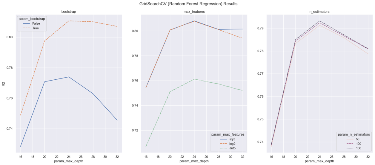Figure 4: GridSearchCV (Random Forest Regression) Results

The information that can be inferred from Figure 4 are,

• The ‘max_depth’ hyperparameter has a noticeable effect on the model’s performance, as shown by the consistent rise and eventual decrease of the R² value. Careful consideration is required when choosing the appropriate value for ‘max_depth,’ as values that are excessively high or low can negatively impact the model’s performance.

• The choice of implementing ‘bootstrap’ or not in the model is very crucial as results show that opting for ‘bootstrap’ can significantly boost the performance of the model.

• The use of the ‘auto’ value for the ‘max_features’ parameter should be strictly avoided, as it clearly shows a significant decline in performance. On the contrary, the ‘sqrt’ and ‘log2’ values exhibit similar performance trends while being approximately three times faster in terms of fitting time compared to ‘auto,’ as shown in Figure 5 below.

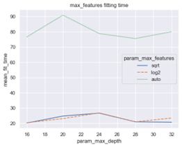Figure 5: Parameter ‘max features’ Fitting Time

• The ‘n_estimators’ hyperparameter demonstrates a consistent impact across its three parameter values. Each value shows a linear increase in R² with increasing ‘max_depth’ until reaching a peak and then declining. After thorough evaluation, a ‘n_estimators’ value of 150 emerges as the optimal choice, although the improvements over the other values are minimal. However, it is important to consider the computational time required, as shown in Figure 6, where the performance gain associated with a ‘n_estimators’ value of 150 comes at a higher computational cost compared to the other two values.

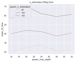Figure 6: Parameter ‘n estimators’ Fitting Time

Using the information presented in Figure 4, 5 and 6, it can be deducted that the best set of hyperparameters to train the Random Forest Regression Model for this project are, ‘bootstrap’ = True, ‘max_depth’ = 24, ‘max_features’ = ‘sqrt’ and ‘n_estimators’ = 150.

XGBoost Regression GridSearchCV

From Figure 3, it is interesting to note that the training time for XGBoost Regression remains constant at around 2 seconds for all sample sizes. This is a remarkably short training time considering the ML model consists of approximately 4 million rows of data. In contrast, Random Forest Regression exhibits a linear relationship between sample size and training time. To minimize training time while maintaining performance, techniques such as sampling can be applied for a GridSearchCV model in Random Forest Regression. However, the same approach is impractical to be applied to XGBoost Regression since its training time remains constant regardless of the sample size. Using the previously mentioned GridSearchCV model with 4 hyperparameters, each having 3 parameters, and applying 5-fold cross-validation to the complete dataset, the training period for XGBoost Regression would be approximately 13.5 minutes. This is significantly lower than the estimated 39 hours required for Random Forest Regression. The selected hyperparameters for the GridSearchCV (XGBoost Regression) model are as follows:

1. max_depth: 6, 8, 10, 12, 14, 16 and 18
2. gamma: 0, 2, 4, 6 and 8.
3. min_child_weight: 0, 5, 10
4. eta: 0.3, 0.5, 0.7 and 0.9
5. verbose: 3. This is to ensure sufficient amount of information regarding the training process is printed.
6. cv: 5. This is the parameter that enables 5-fold cross validation

The results of the GridSearchCV (XGBoost Regression) Model from the steps above are shown in Figure 7 below,

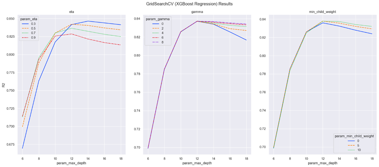Figure 7: GridSearchCV (XGBoost Regression) Results

The information that can be deduced from Figure 7 are,

• The hyperparameter ‘max_depth’ plays a crucial role in determining the performance of the XGBoost model. It has a direct impact on the R² value, initially increasing linearly before reaching a peak and subsequently declining in performance.
• The hyperparameter ‘eta’ has a unique behaviour among its parameters. 0.5, 0.7 and 0.9 seems to exhibit a similar trend of rising linearly with R², reaching a peak point, and steeply declining in performance. 0.3 stands out by showing similar trends as the other values but seems to have a lagging phase in reaching its peak point.
• In terms of the hyperparameter ‘gamma’, all parameter values display the same behaviour before reaching the peak point with R². After the peak point, the lower the ‘gamma’ value, the steeper it declines in performance.
• The hyperparameter ‘min_child_weight’ exhibits the same trend as ‘gamma’ although much more pronounced here.

From the charts in Figure 7, it can be inferred that the best set of hyperparameters to train the GridSearchCV (XGBoost Regression) model are ‘eta’ = 0.3, ‘max_depth’ = 14, ‘gamma’ = 4 and ‘min_child_weight’ = 10.

Analysis and Evaluation

Using the best set of hyperparameters from the previous GridSearchCV models for both Random Forest Regression and XGBoost Regression, the final ML models were developed on the complete dataset, and the results comparison are illustrated in Figure 8 below.

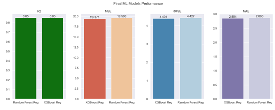Figure 8: Final ML Models Performance

Based on the findings presented in Figure 8, there is minimal difference in performance evaluation metrics between the two models. Both machine learning models were able to surpass the widely accepted R² score of 0.8, achieving a precise value of 0.85 for this project. Upon examining the error metrics, XGBoost Regression demonstrated fewer errors across all three metrics (MSE, RMSE, and MAE) compared to the other model, although the difference between the two is negligible. Additionally, Figure 9 sheds light on the computational time needed to evaluate the performance of the models.

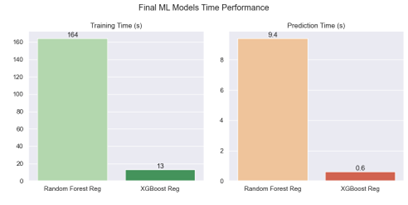Figure 9: Final ML Models Time Performance

As shown in Figure 9, XGBoost Regression performed better than Random Forest Regression, delivering similar results while significantly reducing computation time by approximately 92%. Additionally, Figure 10 highlights another advantage of XGBoost Regression which is the smaller size of its machine learning model.

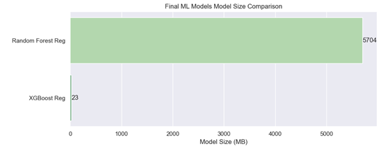Figure 10: Final ML Models Size Comparison

Figure 10 shows that XGBoost Regression has a significantly smaller ML Model size compared to Random Forest Regression, being almost 99.6% smaller. Based on the insights from Figures 8, 9, and 10, it can be concluded that XGBoost Regression is the superior model, not only in terms of performance metrics but also in computational efficiency, with shorter training time and a smaller ML model size. Additionally, the feature importance plot for XGBoost Regression in Figure 11 highlights the three most important predictors of crime rate which are Crime Score, LE Score, and Income Score.

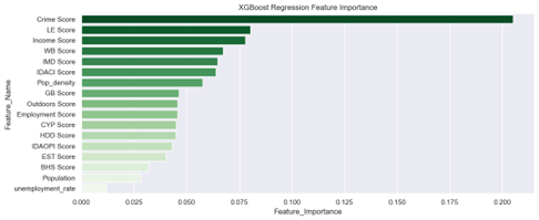Figure 11: XGBoost Regression Feature Importance Plot

The Python scripts to perform the benchmark, ML model developments, GridSearchCV models and performance evaluations mentioned in this article are hosted in my Github Repo